Discovering Physical Equations

This example shows how ndCurveMaster can be used to discover physical equations from data.

This tutorial includes three examples:

1. the relationship between acceleration, distance, and time,
2. the equivalent resistance equation,
3. Coulomb's law.

In all examples, the proper selection of base functions is crucial. The goal is to limit the function set to forms that may lead to the discovery of a real physical relationship.

1. Discovering the acceleration equation

We load the file Acceleration.txt, which you can download here: Acceleration.txt. The file contains values of distance, time, and acceleration calculated on the basis of distance and time.

As the dependent variable Y, we choose a, while as the independent variables X, we choose s and t.

We select the Add combination of X variables option so that the program also includes combinations of the X variables.

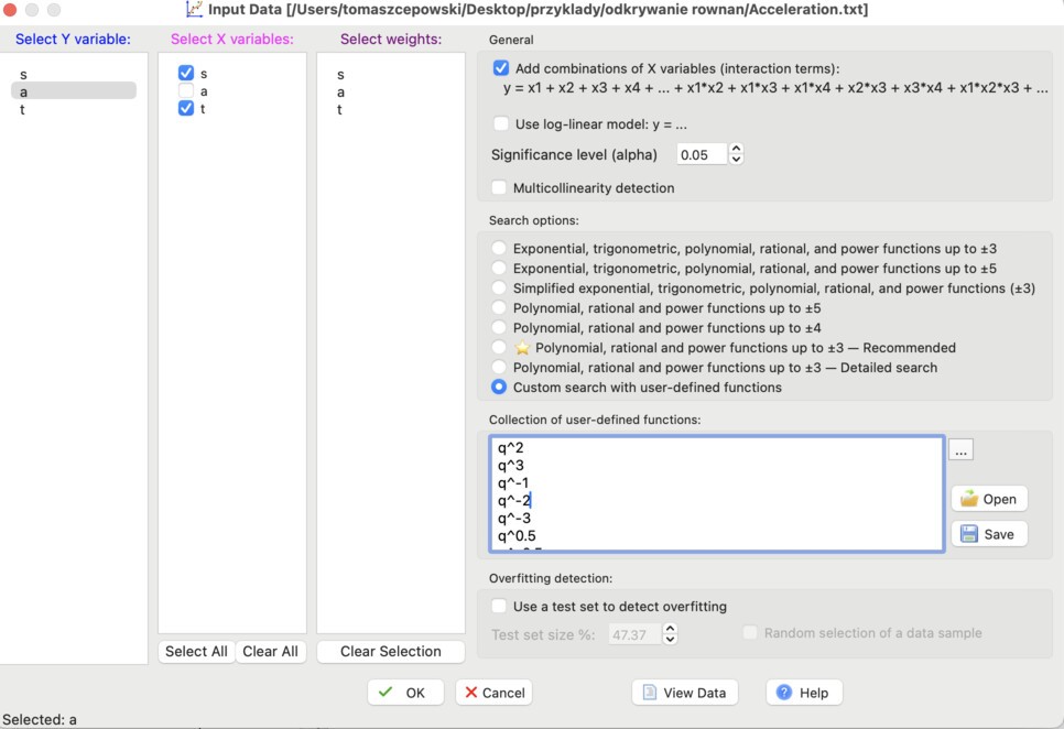
A key step is preparing a custom set of functions that contains only the basic functions needed to discover physical relationships. To do this, in the Search options field we choose Custom search with user-defined functions and enter the following functions:

The symbol q represents a variable.

Details about custom functions are described here:

https://www.ndcurvemaster.com/help-882/custom_collection.html

We do not select the Multicollinearity detection option or any options related to overfitting detection.

At the beginning, a window appears with a linear model that also includes combinations of variables:

In the Settings window, we clear all search-criteria filters:

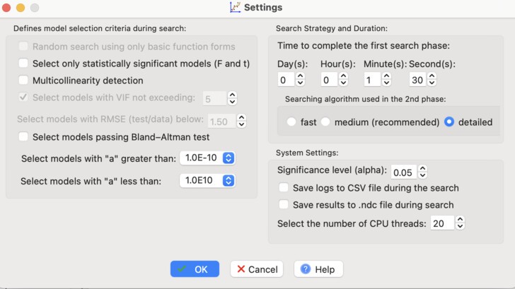
In the Search Strategy section, we extend the duration of the first search phase to 1 minute and 30 seconds, and we enable the detailed iterative algorithm for the second phase.

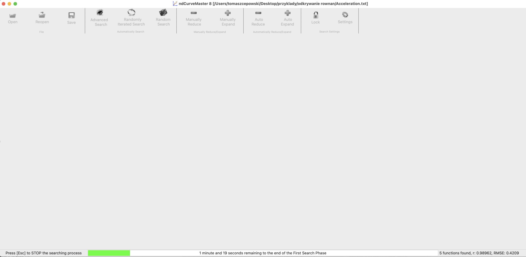
After closing the Settings window, we click the Advanced Search button.

A search window should appear:

Then a list of discovered equations appears:

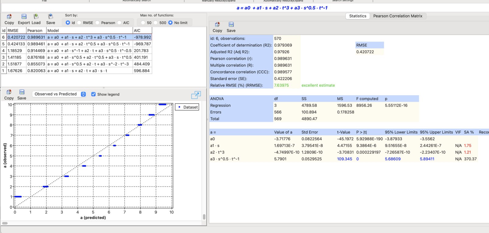
The predictors of the most accurate equation have the following statistics:

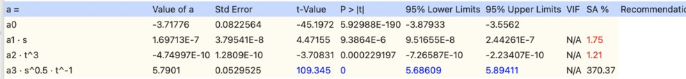
It can be seen that the last predictor, s^-0.5*t^-1, has the highest SA% value, whereas the SA% values for the other predictors are much lower. This means that this predictor may represent the correct physical relationship.

Now the model should be simplified by keeping only this significant predictor. We also remove the constant term a0, because we are looking for a physical equation without a constant.

To do this, we click the Manually Reduce button, and in the new window we select the predictor of interest and clear the others:

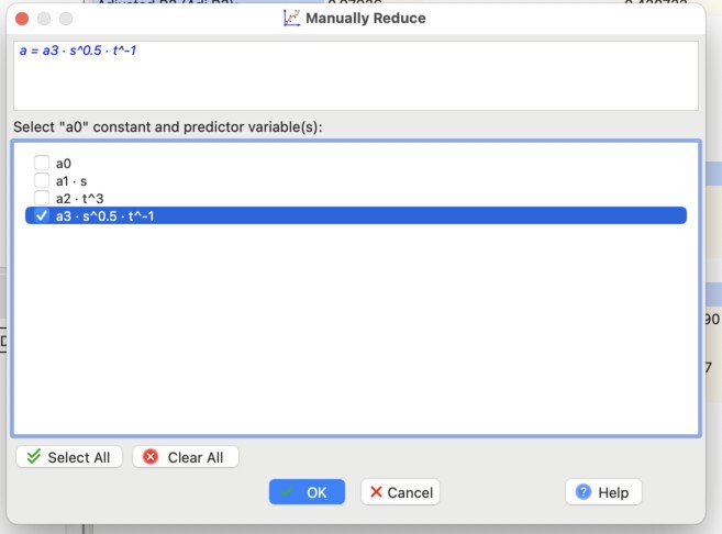
After confirmation, the following model appears:

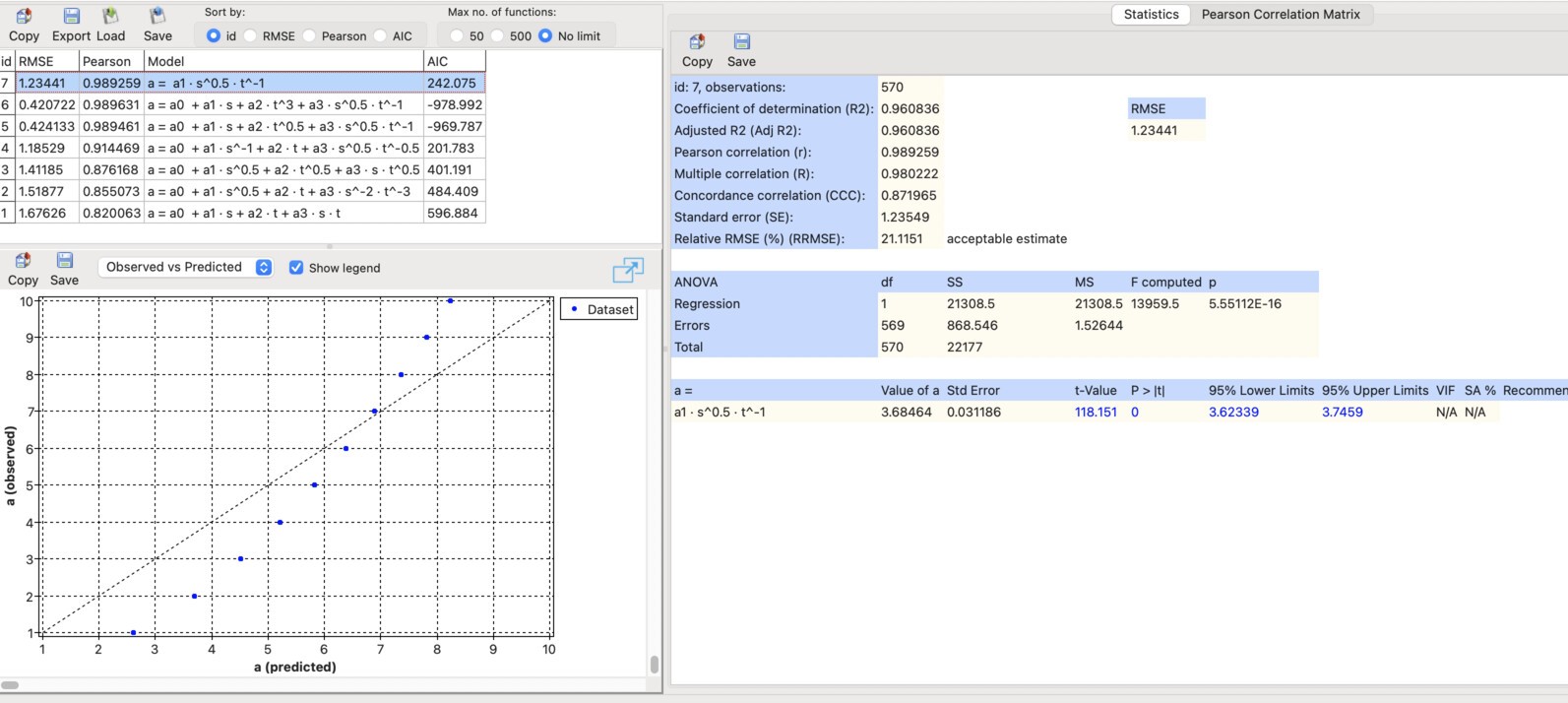
Next, we click the Random Search button.

After some time, the following solution should appear:

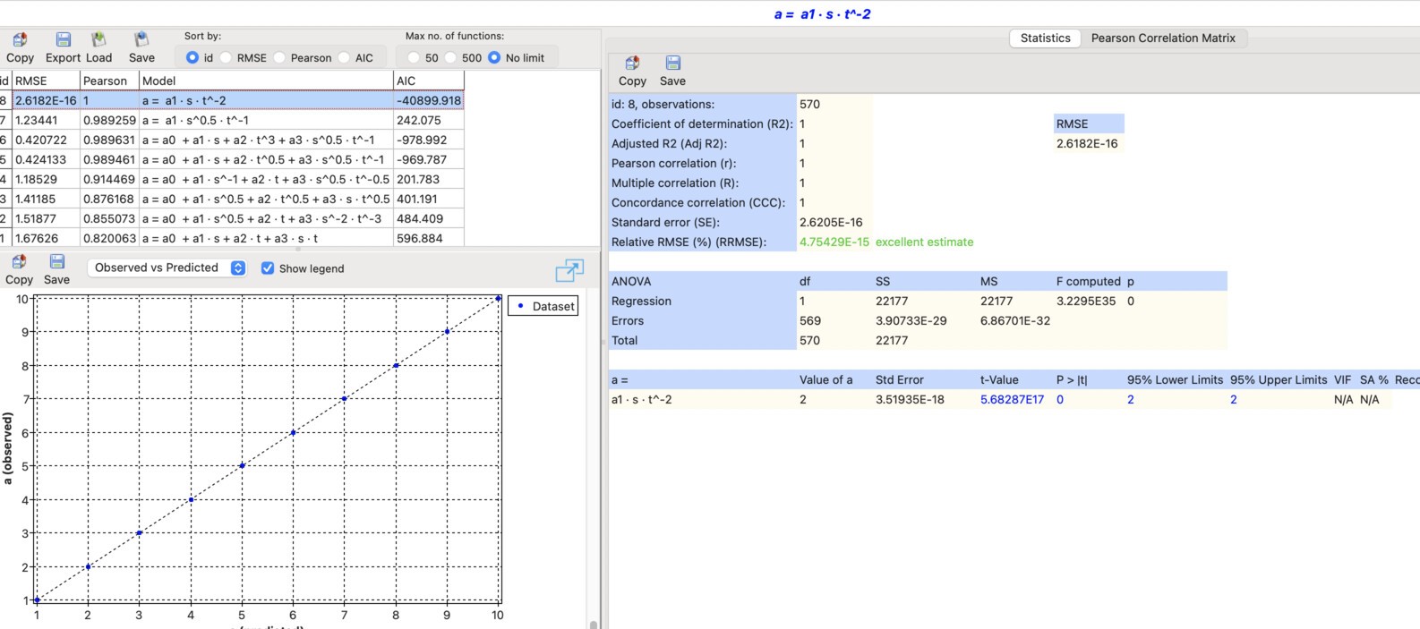
As can be seen, the program found the correct relationship between acceleration a, distance s, and time t:

2. Discovering the equivalent resistance equation

Now, using the same method, we will discover the resistance equation. To do this, we load the file Resistance.txt, which you can download here: Resistance.txt, and choose the following settings:

As Search options, we choose the same function set as in the previous example.

Next, we click OK, and then the Advanced Search button.

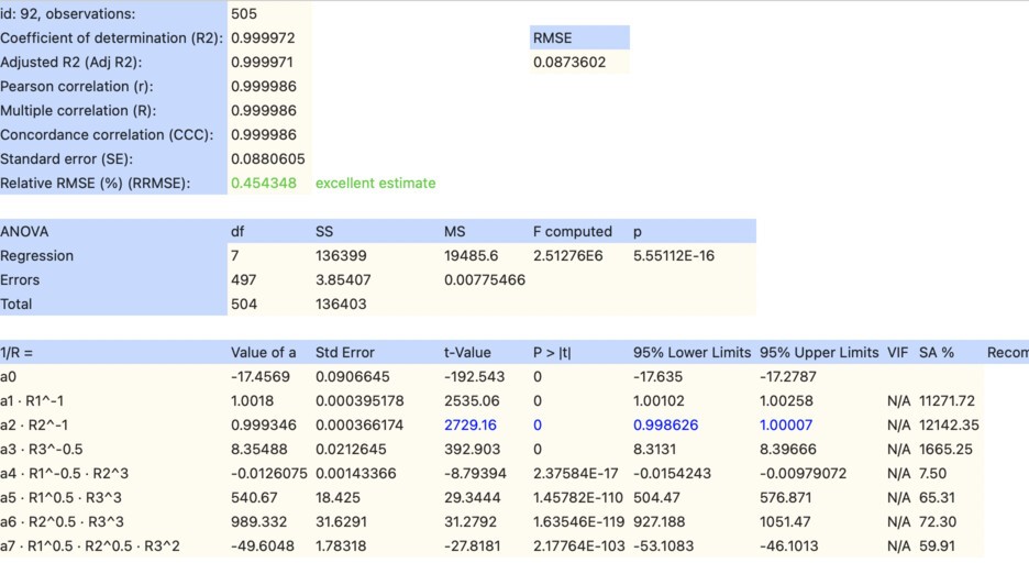
After the specified time has elapsed, a window appears showing the model results for resistance.

It can be seen that in equation id: 92, the most important predictors are R1^-1, R2^-1, and R3^-0.5. For these predictors, the SA% indicator is significantly higher than for the others:

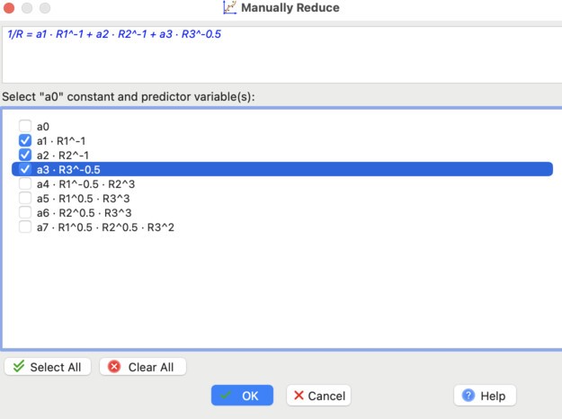
Therefore, we keep only these three predictors and remove the others by clicking the Manually Reduce button:

Next, we click the Random Search button.

After finding the optimal equation id: 94, the program stops the calculations. The result is shown below:

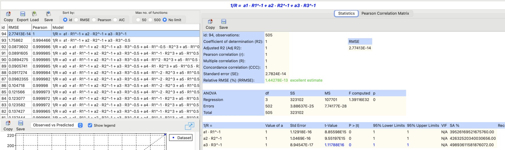
It can be seen that ndCurveMaster found the correct resistance equation:

3. Discovering Coulomb's law from data

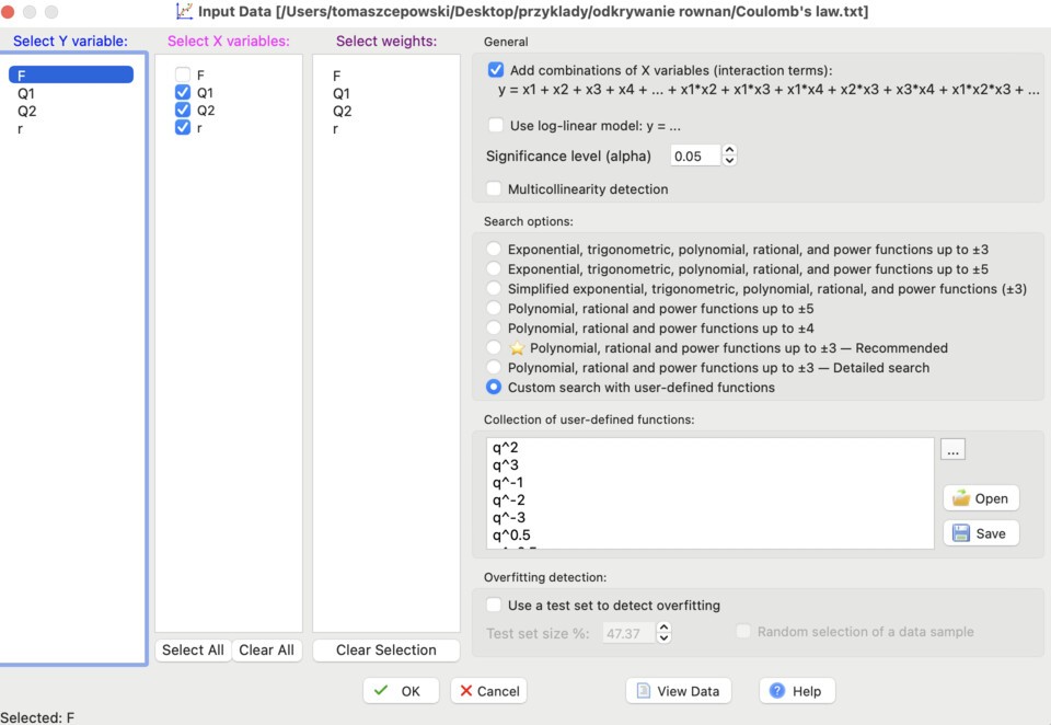
Now we will discover Coulomb's law from data. We load the file Coulomb's_law.txt, which you can download here: Coulomb's_law.txt, and use the same settings as in the previous examples:

After loading the data, we click Advanced Search. After a moment, the following solution appears:

It is clearly visible that in model id: 75, the last predictor is the most significant.

We click the Manually Reduce button and select only this predictor:

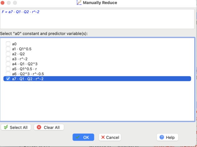
There is no need to continue the search using Random Search, because the discovered model already represents Coulomb's law:

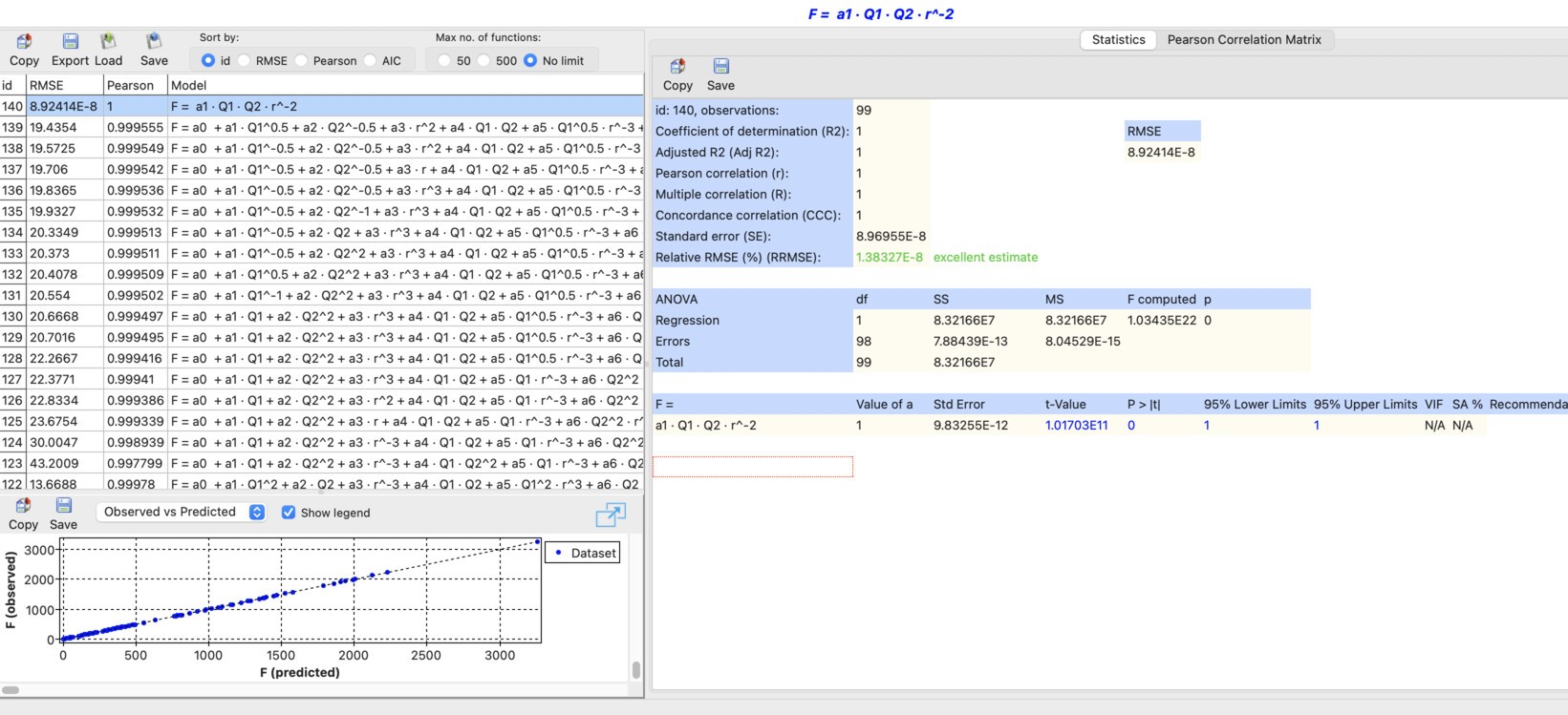
The obtained equation has the following form: