Calculating Constants of Differential Equations
Sometimes it is necessary to determine the constants of the general solution of a differential equation on the basis of measurements, especially when the boundary conditions are unknown or unclear.
This example shows how, knowing the general form of the solution and having measurement data, the constants of the equation can be determined using ndCurveMaster. Of course, such constants can also be calculated with other tools, but in ndCurveMaster this can be done in a simple and convenient way.
Let us assume that the deflection of an elastic beam was measured and the results were saved in the file Beam.txt, which you can download here: Beam.txt.
The equation describing this deflection is known:
EI d4y / dx4 + ky = 0 (1)
as well as its general solution:
y(x) = C1 cos x + C2 sin x + C3 cosh x + C4 sinh x (2)
The goal is to determine the constants C1–C4 of this solution.
1. Loading the data and initial settings
After loading the file Beam.txt, enter the following settings:
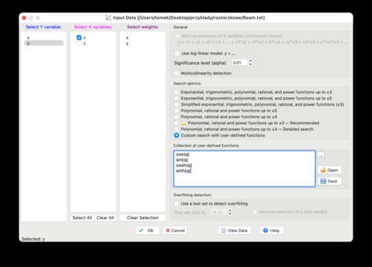
It is important to select Custom search with user-defined functions in the Search options field and enter the following functions:
sin(q)
cosh(q)
sinh(q)
Details about this option are described here:
https://www.ndcurvemaster.com/help-882/custom_collection.html
After loading the data, a window with the basic linear model will appear:
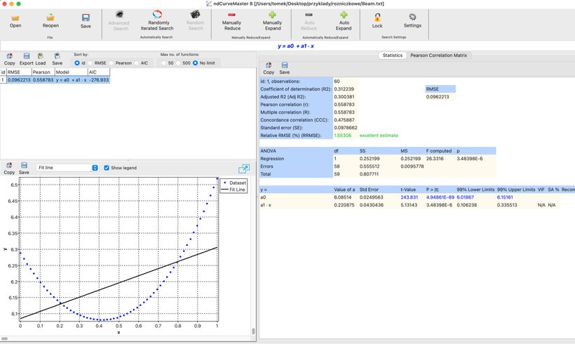
This model must be replaced with the model resulting from the general solution of the equation. This means that four predictors need to be added: cos(x), sin(x), cosh(x), and sinh(x).
2. Adding the appropriate predictors
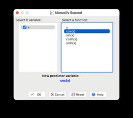
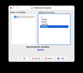
To do this, click the Manually Expand button and add the indicated predictors one by one, confirming each selection by clicking OK.
Step 1
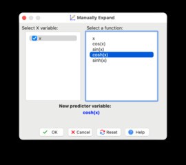
Step 2

Step 3
Step 4
After adding these predictors, the model will look as follows:

3. Reducing the model
Now it is enough to remove the constant term a0 and the predictor x1 from the model. To do this, click the Manually Reduce button and deselect these two elements, as shown in the figure:
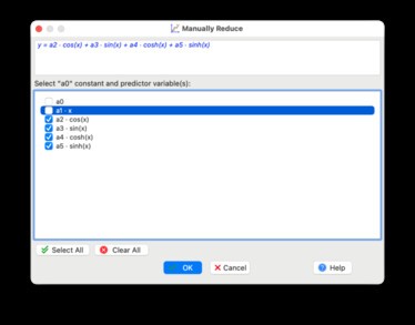
Then click OK.
As a result, you will obtain the following model id: 6:
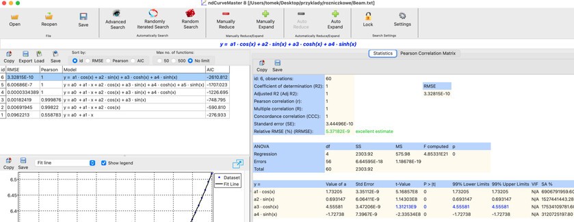
The equation of this model is:
The regression coefficients of this model are, of course, the constants C1–C4 from the general solution of the equation, namely:
C2 = 0.693147182595567
C3 = 4.55580621799891
C4 = -1.72737909437274
ndCurveMaster project file
You can download the ndCurveMaster project file for this example here: Beam.ndc