4D Curve Fitting: From Polynomial to Optimized Nonlinear Model

In the previous example, we fitted a curve f(x) to data. In this example, we fit a function of three input variables, that is, f(x1, x2, x3), using a polynomial model and then improve it with an optimized nonlinear model.

In other words, we build a 4D curve fitting model with three inputs and one output. This is an example of multivariable curve fitting and multivariable nonlinear regression.

After launching ndCurveMaster, load the file CurveFitting4D.txt, which you can download here: CurveFitting4D.txt.

Next, apply the following settings:

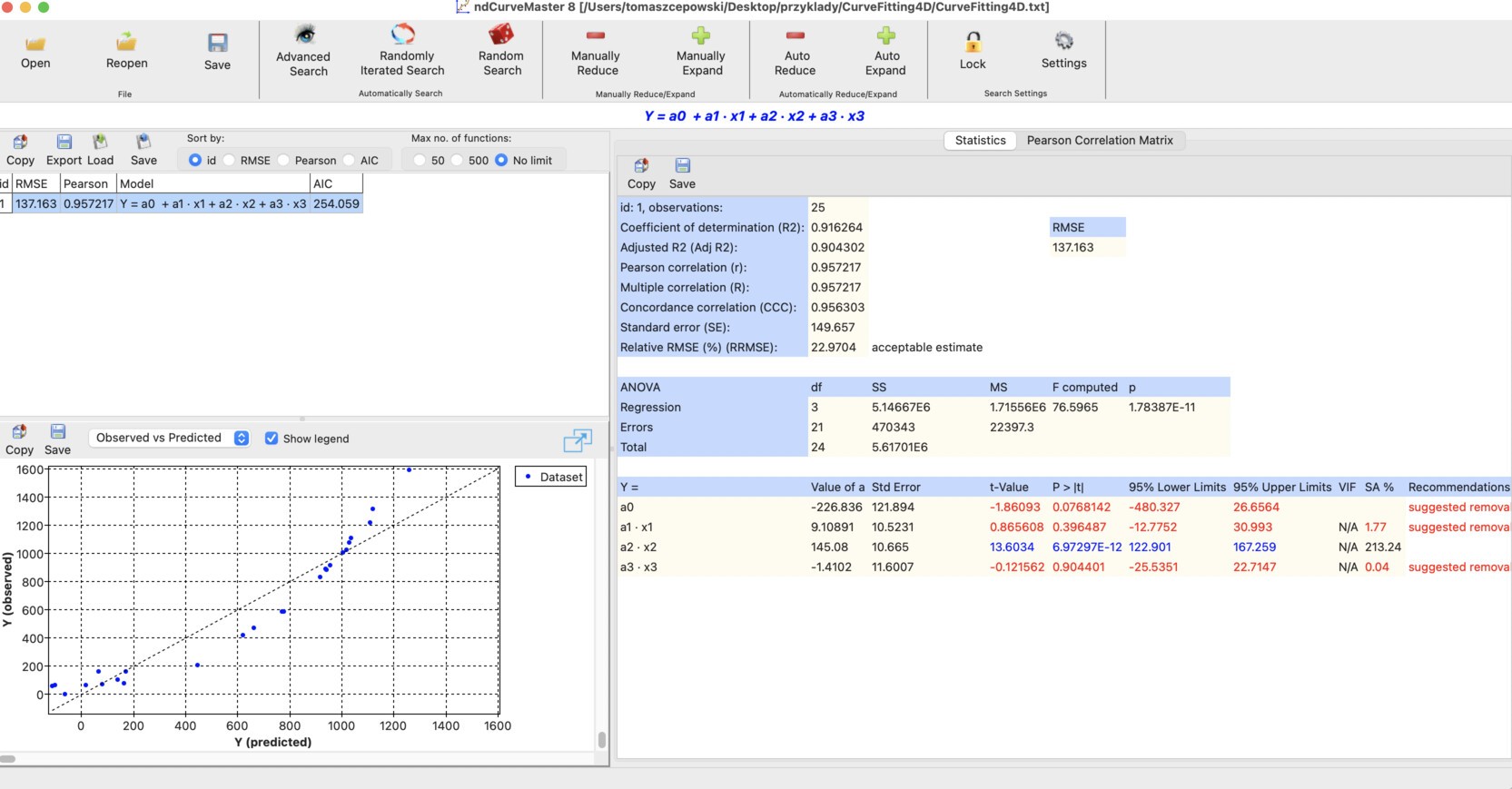
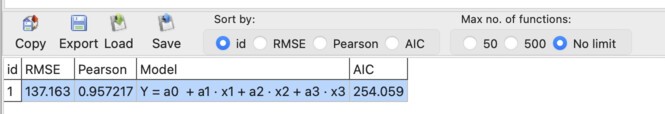
After loading the data, a basic linear model with three independent variables x1, x2, and x3 is obtained:

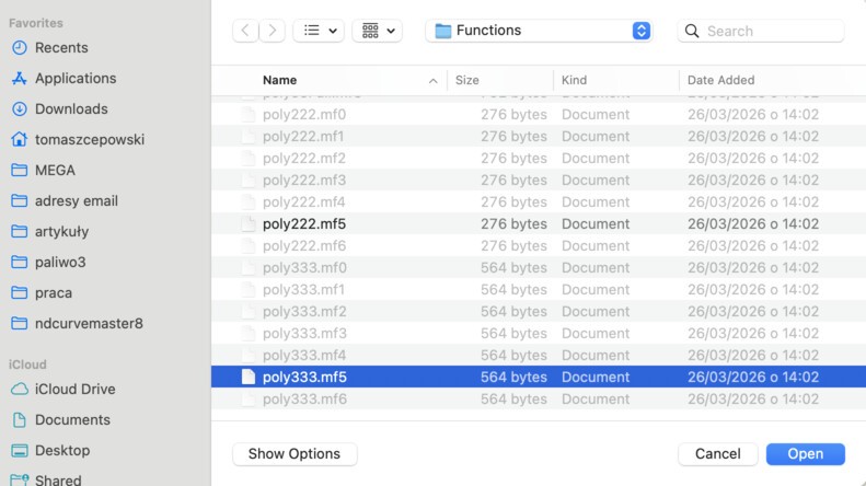
Next, click the Load button located above the model list in the upper-left panel of the program:

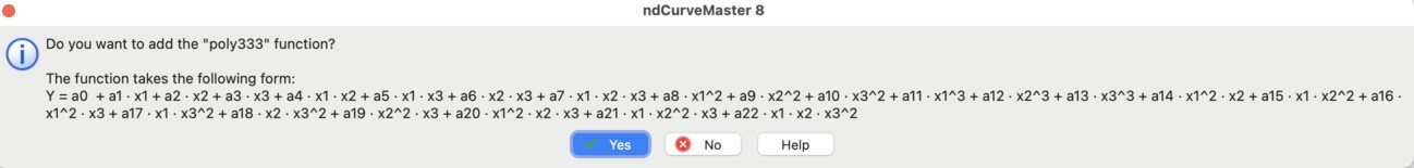
Load the polynomial model poly333.mf5:

This is a third-degree polynomial model. More information about this function and available model sets can be found here: https://www.ndcurvemaster.com/help-882/functions.html

After selecting this model, confirm the selection:

As a result, the following third-degree polynomial function is obtained:

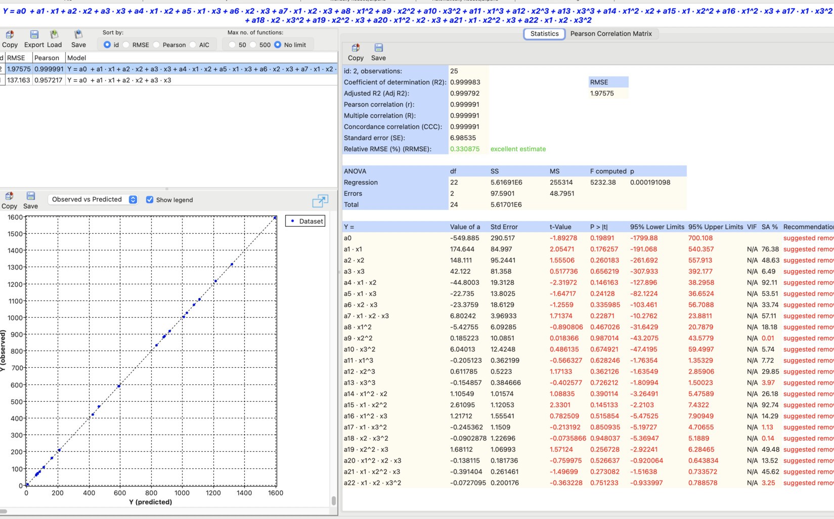
The function fits the data reasonably well; however, some predictors are not statistically significant.

We will now perform a more thorough search to obtain a more accurate model. Before starting the search, apply the following settings:

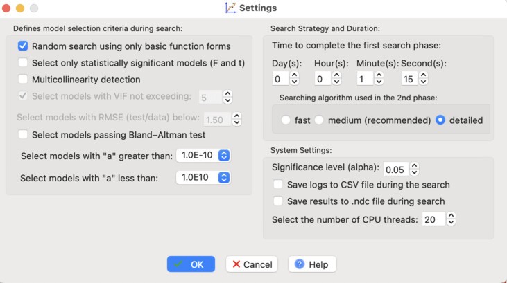
Enabling the Random search using only basic forms option ensures that only basic functional forms are explored during the random search phase. In the second, iterative phase, more detailed functions are identified. This approach allows the algorithm to first find general solutions and then refine them, which can improve efficiency.

Set the duration of the first search phase to 1 minute and 15 seconds.

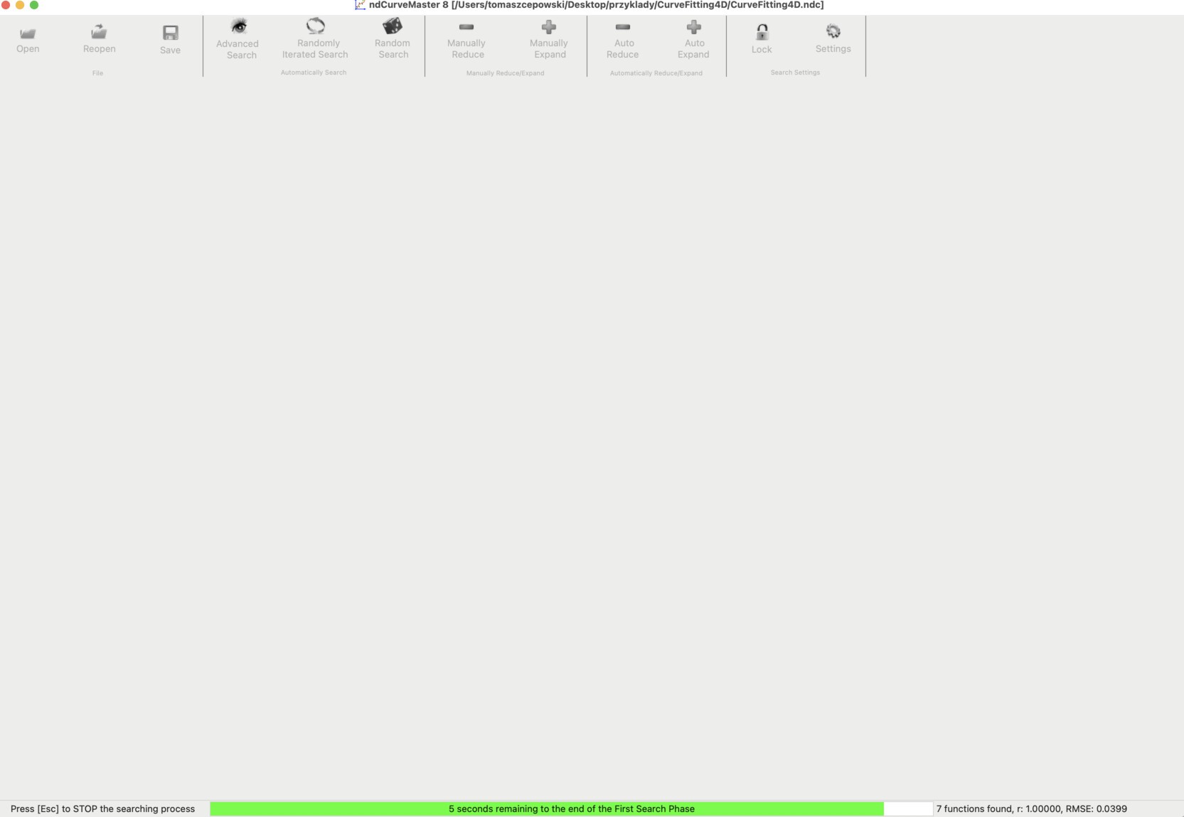
Then click Advanced Search to start the search process.

As shown, at least seven general models were discovered in the first search phase:

These models are shown below:

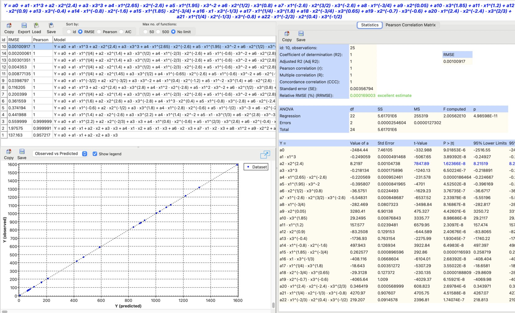
The remaining models are more detailed. The most accurate one is model id: 10:

For comparison, model id: 2 (a third-degree polynomial) has the following form:

For this model, RMSE = 1.97575.

In contrast, the optimized model id: 10 achieves RMSE = 0.00100917.

Interestingly, the statistical significance of all predictors has also improved.

The final form of model id: 10 is:

As shown, ndCurveMaster effectively optimized the exponents of the predictors from model id: 2. This example demonstrates that multivariable nonlinear curve fitting can substantially improve model accuracy compared with a standard polynomial model.